
Fast and Memory Efficient Algorithms for Time–Frequency Distributions
Contents
download
download fast_TFDs (or fork on github)
overview
A collection of M-files to compute time–frequency distributions from the quadratic class [1]. Memory and computational load is limited by controlling the level of over-sampling for the TFD. Oversampling in the TFD is proportional to signal length and bandwidth of the Doppler–lag kernel. Algorithms are optimised to four kernel types: nonseparable, separable, lag-independent, and Doppler-independent kernels.
Also included are algorithms to compute decimated, or sub-sampled, TFDs. Again, these algorithms are specific to the four kernel types but compute approximate TFDs by a process of decimatation.
This package was meanst to replace the fast TFDs package as is better programmed to save memory and is simplier to use. The code at fast TFDs however, is specific to the reference [2] whereas this code is more general and (should be) easier to use.
Requires Matlab or Octave (programming environments).
quick start
First, add paths using the load_curdir function:
>> load_curdir;description
There are two sets of TFD algorithms: one set computes oversampled TFDs and the other set computes decimated (sub-sampled or undersampled) TFDs. The first set, for computing oversampled TFDs, has four algorithms for specific kernel types, namely the - non-separable kernel, - separable kernel, - Doppler-independent (DI) kernel, - and lag-independent (LI) kernel.
The function to generate these oversampled TFDs is full_tfd.m. The following
examples, using a test signal, illustrates usage:
% generate test signal:
  N=512;
  x=gen_LFM(N,0.1,0.3) + gen_LFM(N,0.4,0.04);

  % nonseparable kernel (Choi-Williams kernel):
  tf=full_tfd(x,'nonsep',{'cw',10});
  figure(1); clf; vtfd(tf,x);

  % separable kernel:
  tf=full_tfd(x,'sep',{ {51,'hann'},{101,'hann'} },256,256);
  figure(2); clf; vtfd(tf,x);

  % Doppler-independent kernel:
  tf=full_tfd(x,'DI',{101,'hann'},256,[]);
  figure(3); clf; vtfd(tf,x);

  % lag-independent kernel:
  tf=full_tfd(x,'LI',{51,'hann'},[],256);
  figure(4); clf; vtfd(tf,x);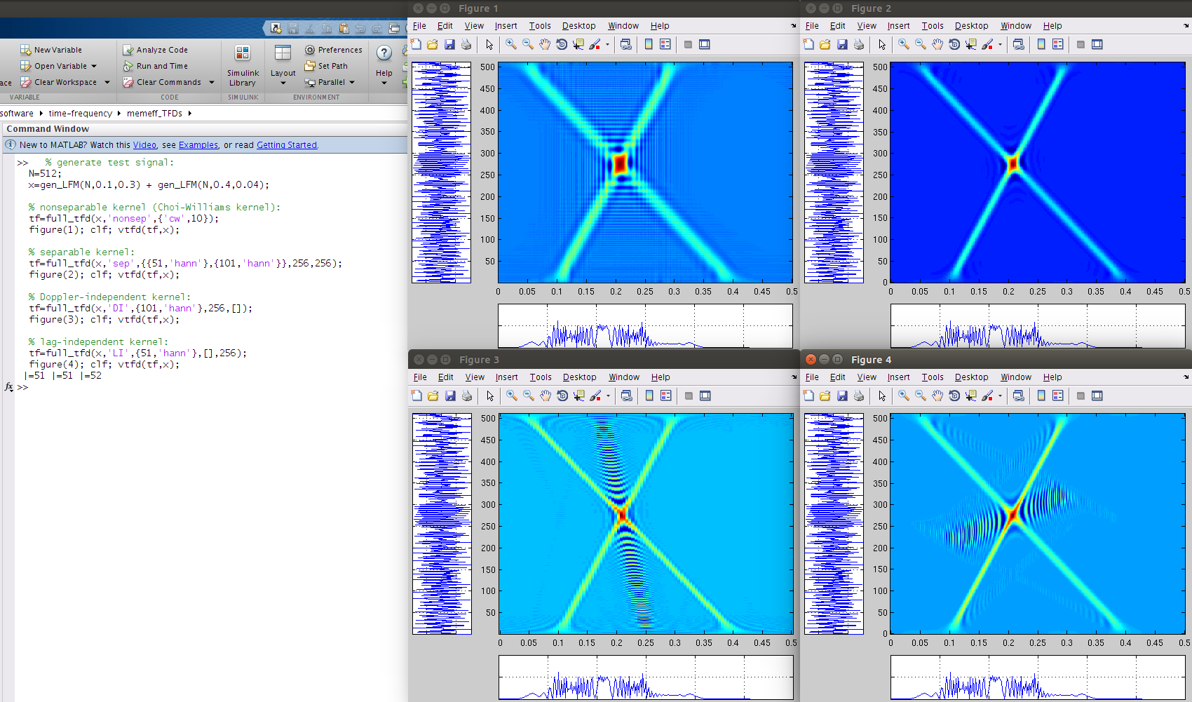
Type help full_tfd for more details.
Likewise, the algorithms for decimated TFDs are specific to the four kernel types. The
function dec_tfd computes the decimated TFDs, as the following examples show:
N=1024; Ntime=64; Nfreq=128;
  a=2; b=2;
  ni=[100:2:900]; ki=[150:2:850];

  x=gen_LFM(N,0.1,0.3)+gen_LFM(N,0.4,0.1);

  % non-separable kernel:
  tf=dec_tfd(x,'nonsep',{'cw',100},N,N,a*4,b*4);
  figure(1); clf; vtfd(tf,x);

  % separable kernel:
  tf=dec_tfd(x,'sep',{ {51,'hann'},{101,'hann'} },Ntime,Nfreq,a,b);
  figure(2); clf; vtfd(tf,x);

  % Doppler-independent kernel:
  tf=dec_tfd(x,'DI',{101,'hann'},N,Nfreq,ni,b);
  figure(3); clf; vtfd(tf,x,1,ni);

  % lag-independent kernel:
  tf=dec_tfd(x,'LI',{51,'hann'},Ntime,N,a,ki);
  figure(4); clf; vtfd(tf,x,1,[],ki./(N*2));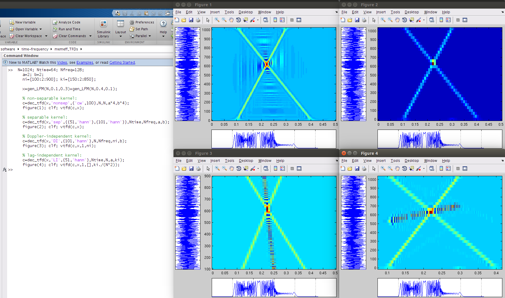
Type help dec_tfd for more details on this function.
files
All Matlab files (.m files) have a description and an example in the header. To read this
header, type help <filename.m> in Matlab. Directory structure is as follows:
├── common             # directory: files to generate kernel functions
├── decimated_TFDs     # directory: files to generate decimated TFD for the 4 kernel types
├── dec_tfd.m          # file: compute decimated TFDs
├── full_tfd.m         # file: compute oversampled TFDs
├── full_TFDs          # directory: files to generate oversampled TFD for the 4 kernel types
├── LICENCE.md         # file: licence file
├── load_curdir.m      # file: adds paths for matlab/octave
├── README.md          # file: this README file
└── utils              # directory: miscellaneous files
computational load
The computational load is measured in terms of the number of FFTs required to compute the TFD. Memory load is measured as number of real-valued numbers required to compute and store the TFD. The real-valued signal (i.e. input signal) is of length N.
Computational load for the oversampled TFDs (using full_tfd.m) is as follows for the
four kernel types:
| kernel-type | computational load | memory |
|---|---|---|
| non-separable | 3N²/2 log₂ N | N² |
| LI | NNtime/2 log₂ Ntime | Ntime × N |
| DI | NNfreq/2 log₂ Nfreq | N × Nfreq |
| separable | Pₕ(N log₂N +Ntime log₂Ntime) | Ntime × Nfreq |
| + NtimeNfreq/2 log₂ Nfreq |
assuming the FFT of length-N signal requires Nlog₂N computations and using the notation:
| symbol | explanation |
|---|---|
| N | length of signal |
| Ntime | length of TFD in time direction |
| Nfreq | length of TFD in frequency direction |
| Pₕ | Pₕ = P/2, where P is the length of the lag window |
And for the decimated TFDs (using dec_tfd.m):
| kernel-type | computational load | memory | grid |
|---|---|---|---|
| non-separable | N²/2 log₂ N + LJ/2 log₂ J | L × J | ρ[an,bn] |
| LI | VLtime/2 log₂ Ltime | Ltime × V | ρ[an,kᵢ] |
| DI | UJfreq/2 log₂ Jfreq | U × Jfreq | ρ[nᵢ,bk] |
| separable | JfreqN/2 log₂N | Ltime × Jfreq | ρ[an,bn] |
| + LtimeJfreq log₂ LtimeJfreq |
using the extra notation:
| symbol | explanation |
|---|---|
| U | length of sequence nᵢ {nᵢ for 1<=i<=U}, U<=N and 0<=nᵢ<=N-1 |
| V | length of sequence kᵢ {kᵢ for 1<=i<=V}, V<=N and 0<=kᵢ<=N-1 |
| J | N/b, b is decimation integer in frequency direction |
| L | N/a, a is decimation integer in time direction |
| Jfreq | Nfreq/b, b is decimation integer in frequency direction |
| Ltime | Ntime/a, a is decimation integer in time direction |
requirements
Either Matlab (R2012 or newer, Mathworks website) or Octave (v3.6 or newer, Octave website, with the ‘octave-signal’ add-on package).
test computer setup
- hardware: Intel(R) Xeon(R) CPU E5-1603 0 @ 2.80GHz; 8GB memory.
- operating system: Ubuntu GNU/Linux x86_64 distribution (Trusty Tahr, 14.04), with Linux kernel 3.13.0-27-generic
- software: Octave 3.8.1 (using Gnuplot 4.6 patchlevel 4), with ‘octave-signal’ toolbox and Matlab (R2009b, R2012a, and R2013a)
licence
Copyright (c) 2014, John M. O' Toole, University College Cork
All rights reserved.

Redistribution and use in source and binary forms, with or without modification,
are permitted provided that the following conditions are met:

  Redistributions of source code must retain the above copyright notice, this
  list of conditions and the following disclaimer.

  Redistributions in binary form must reproduce the above copyright notice, this
  list of conditions and the following disclaimer in the documentation and/or
  other materials provided with the distribution.

  Neither the name of the University College Cork nor the names of its
  contributors may be used to endorse or promote products derived from
  this software without specific prior written permission.

THIS SOFTWARE IS PROVIDED BY THE COPYRIGHT HOLDERS AND CONTRIBUTORS "AS IS" AND
ANY EXPRESS OR IMPLIED WARRANTIES, INCLUDING, BUT NOT LIMITED TO, THE IMPLIED
WARRANTIES OF MERCHANTABILITY AND FITNESS FOR A PARTICULAR PURPOSE ARE
DISCLAIMED. IN NO EVENT SHALL THE COPYRIGHT HOLDER OR CONTRIBUTORS BE LIABLE FOR
ANY DIRECT, INDIRECT, INCIDENTAL, SPECIAL, EXEMPLARY, OR CONSEQUENTIAL DAMAGES
(INCLUDING, BUT NOT LIMITED TO, PROCUREMENT OF SUBSTITUTE GOODS OR SERVICES;
LOSS OF USE, DATA, OR PROFITS; OR BUSINESS INTERRUPTION) HOWEVER CAUSED AND ON
ANY THEORY OF LIABILITY, WHETHER IN CONTRACT, STRICT LIABILITY, OR TORT
(INCLUDING NEGLIGENCE OR OTHERWISE) ARISING IN ANY WAY OUT OF THE USE OF THIS
SOFTWARE, EVEN IF ADVISED OF THE POSSIBILITY OF SUCH DAMAGE.
references
-
J.M. O’ Toole and B. Boashash, “Memory Efficient Algorithms for TFDs”, Article 6.6, Chapter 6, in Time–Frequency Signal Processing and Analysis: A Comprenhensive Reference, Second Edition, 2014, in press.
-
J.M. O’ Toole and B. Boashash, “Fast and memory-efficient algorithms for computing quadratic time–frequency distributions”, Applied and Computational Harmonic Analysis, vol. 35, no. 2, pp. 350–358, 2013.
-
J.M. Oʼ Toole, M. Mesbah, and B. Boashash, “Improved discrete definition of quadratic time–frequency distributions,” IEEE Transactions on Signal Processing, vol. 58, Feb. 2010, pp. 906-911.
-
J.M. O’ Toole, M. Mesbah, and B. Boashash, “A New Discrete Analytic Signal for Reducing Aliasing in the Discrete Wigner-Ville Distribution”, IEEE Transactions on Signal Processing, vol. 56, no. 11, pp. 5427-5434, Nov. 2008.
-
J.M. Oʼ Toole, M. Mesbah, and B. Boashash, “Algorithms for discrete quadratic time–frequency distributions,” WSEAS Transactions on Signal Processing, vol. 4, May. 2008, pp. 320-329.
contact
John M. O’ Toole
Neonatal Brain Research Group,
Irish Centre for Fetal and Neonatal Translational Research (INFANT),
Department of Paediatrics and Child Health,
University College Dublin,
Western Gateway Building, Room 2.17,
Cork, Ireland
- email: j.otoole
ieee.org - web: http://otoolej.github.io/