Algorithms for (Quadratic) Time–Frequency Distributions

Download
Overview
Quick Start
Examples
References

IMPORTANT: this code accompanies the paper [1]; for a newer and more user-friendly package please use the memory-efficient TFD package.

Download

download fast_TFDs (or fork on github)

Overview

This collection of M-files generate time-frequency distributions (TFDs) with as few computations and as little memory as possible. The algorithms are described in [1]; the discrete TFD definition they compute is in [2].

There are two sets of algorithms. The first set (Set1) computes the exact TFD and minimises on oversampling. The second set (Set2) computes a decimated TFD, and therefore is not exact but may be useful for some applications.

Each set computes four different types of kernels:

nonseparable kernel
separable kernel
Doppler-independent kernel
lag-independent kernel

(see [1] for more details). Code is organised in folders as follows:

fast_TFDs/
├── full_DTFD/     # Set1 algorithms: compute exact TFDs
│   └── .m files
├── dec_DTFD/      # Set2 algorithms: compute decimated TFDs
│   └── .m files
├── utils/         # extra functions 
│   └── .m files 
└── common/        # common functions used by Set1 and Set2 algorithms
    └── .m files

These programs should run in either Matlab (v7.9.0) or Octave (v3.2.4)

Quick Start

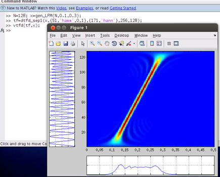
To start, in Matlab (or Octave) load the paths:

>> load_paths_DTFDs;

Next, generate a test signal:

>> N=128; x=gen_LFM(N,0.1,0.3);

Second, generate a TFD with a separable kernel:

>> tf=dtfd_sep1(x,{51,'hamm',0,1},{171,'hann'},256,128);

Third, plot the TFD:

>> vtfd(tf,x);

LFM example — Separable-kernel distribution generated with a linear frequency modulated signal (in Matlab environment).

Examples

In all the examples, start by adding the paths by running the command

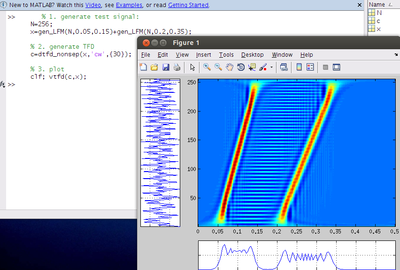
>> load_paths_DTFDs;

Example 1: Choi-Williams

Using the exact-TFD algorithm (from Set1 [1]):

% 1. generate test signal:
      N=256; 
      x=gen_LFM(N,0.05,0.15)+gen_LFM(N,0.2,0.35);

      % 2. generate TFD
      c=dtfd_nonsep(x,'cw',{30}); 

      % 3. plot
      clf; vtfd(c,x);

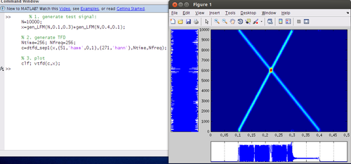
Example 2: Separable-kernel TFD

Using exact-TFD algorithm from Set1 [1]

% 1. generate test signal:
      N=10000; 
      x=gen_LFM(N,0.1,0.3)+gen_LFM(N,0.4,0.1);

      % 2. generate TFD
      Ntime=256; Nfreq=256;
      c=dtfd_sep1(x,{51,'hamm',0,1},{271,'hann'},Ntime,Nfreq); 

      % 3. plot
      clf; vtfd(c,x);

Example 3: Doppler-independent kernel TFD

Using decimated TFD algorithm (from Set2 [1]) generating selective time portions of the signal:

% 1. generate test signal:
      N=171; 
      x=gen_LFM(N,0.1,0.4);

      % 2. generate TFD:
      Nfreq=258; 
      time_dec=[20:3:160,191:250,255,256]; freq_dec=3;
      tf=dec_dtfd_DI(x,{51,'hamm'},Nfreq,time_dec,freq_dec); 

      % 3. plot
      clf; vtfd(tf);

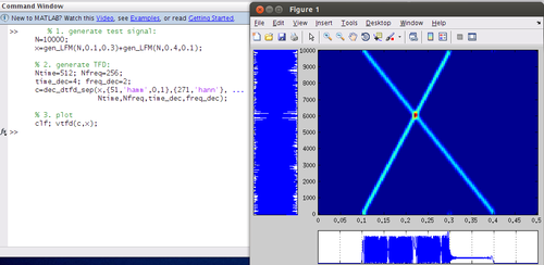
Example 4: Separable kernel TFD

using decimated TFD algorithm from Set2 [1].

% 1. generate test signal:
      N=10000; 
      x=gen_LFM(N,0.1,0.3)+gen_LFM(N,0.4,0.1);

      % 2. generate TFD:
      Ntime=512; Nfreq=256;
      time_dec=4; freq_dec=2;
      c=dec_dtfd_sep(x,{51,'hamm',0,1},{271,'hann'}, ...
                     Ntime,Nfreq,time_dec,freq_dec); 

      % 3. plot
      clf; vtfd(c,x);

Test Computer Setup

hardware: Intel Core Duo CPU, 2.13GHz; 2GB memory.
operating system: Ubuntu GNU/Linux i686 distribution (Natty, 11.04), with Linux kernel 2.6.38-8-generic
software: Octave 3.2.4 (using Gnuplot 4.4 patchlevel 2) and Matlab (R2009b, R2012a, and R2013a)

Copyright

Copyright (c) 2008-2010 John M. O' Toole, The University of Queensland
Copyright (c) 2011-2012 John M. O' Toole, University of Deusto
Copyright (c) 2013 John M. O' Toole, University College Cork
All rights reserved.
Email:  j.otoole@ieee.org

  Redistribution and use in source and binary forms, with or without
  modification, are permitted provided that the following
  conditions are met:
  * Redistributions of source code must retain the above
    copyright notice, this list of conditions and the following
    disclaimer.

  * Redistributions in binary form must reproduce the above
    copyright notice, this list of conditions and the following
    disclaimer in the documentation and/or other materials
    provided with the distribution.
  * Neither the name of the The University of Queensland nor the 
    names of its contributors may be used to endorse or promote 
    products derived from this software without specific prior 
    written permission.
  
  THIS SOFTWARE IS PROVIDED BY JOHN M. O' TOOLE ''AS IS'' AND ANY
  EXPRESS OR IMPLIED WARRANTIES, INCLUDING, BUT NOT LIMITED TO, THE
  IMPLIED WARRANTIES OF MERCHANTABILITY AND FITNESS FOR A PARTICULAR
  PURPOSE ARE DISCLAIMED. IN NO EVENT SHALL JOHN M. O' TOOLE BE
  LIABLE FOR ANY DIRECT, INDIRECT, INCIDENTAL, SPECIAL, EXEMPLARY, OR
  CONSEQUENTIAL DAMAGES (INCLUDING, BUT NOT LIMITED TO, PROCUREMENT
  OF SUBSTITUTE GOODS OR SERVICES; LOSS OF USE, DATA, OR PROFITS; OR
  BUSINESS INTERRUPTION) HOWEVER CAUSED AND ON ANY THEORY OF
  LIABILITY, WHETHER IN CONTRACT, STRICT LIABILITY, OR TORT
  (INCLUDING NEGLIGENCE OR OTHERWISE) ARISING IN ANY WAY OUT OF THE
  USE OF THIS SOFTWARE, EVEN IF ADVISED OF THE POSSIBILITY OF SUCH
  DAMAGE.

Please cite appropriates reference in [1] if you use this software to generate results or prepare data for publication.

References

J.M. O’ Toole and B. Boashash, “Fast and memory-efficient algorithms for computing quadratic time–frequency distributions”, Applied and Computational Harmonic Analysis, Feb. 2013, doi:10.1016/j.acha.2013.01.003
J.M. Oʼ Toole, M. Mesbah, and B. Boashash, “Improved discrete definition of quadratic time–frequency distributions,” IEEE Trans. on Signal Processing, vol. 58, Feb. 2010, pp. 906-911.
J.M. O’ Toole, M. Mesbah, and B. Boashash, “A New Discrete Analytic Signal for Reducing Aliasing in the Discrete Wigner-Ville Distribution”, IEEE Trans. on Signal Processing, vol. 56, no. 11, pp. 5427-5434, Nov. 2008.
J.M. Oʼ Toole, M. Mesbah, and B. Boashash, “Algorithms for discrete quadratic time–frequency distributions,” WSEAS Trans. Signal Processing, vol. 4, May. 2008, pp. 320-329.

J.M. O' Toole